I’ll try and keep this as non-mathematical as possible.

For thermistors (specifically) we now have a much easier way.

What this is about is calculating “weird” functions of a single variable, i.e translating one number into another. A common example in my work is linearizing a thermistor. Other examples might be motor speed versus applied voltage, engine torque versus rpm, the flow rate in a pipe versus pressure, etc. What these all have in common is that the “output” (say flow) is not a linear function of the “input” (say voltage). In fact, you may not even have a formula, just a manually plotted curve.

For example, the curve below is a plot of the air flow in kg/hour (Y axis) versus output voltage of a Mass Air Flow (MAF) sensor used in an engine management system. The curve is clearly very non-linear.

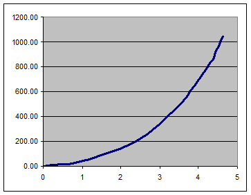
Suppose we need to translate analog input readings into engineering units (kg/hr) according to above curve. Here are the steps.

Step 1. Make sure the horizontal axis represents the value read by the SPLat.

This may sound silly, but often the tendency will be to plot the output of a sensor (volts) on the Y axis versus the measured quantity (say flow) on the X-axis. In the procedure we are using we need the data the other way around. What we know when we perform our calculation is the input variable, and it should be plotted on the X (horizontal) axis.

Step 2. Get the data into an Excel spreadsheet and plot it.

Later on we will be using some magic in Excel to do the really hard work. Use Excel’s Chart function to plot the data as a scatter diagram. Select the format with a smooth line and no data points. You should get something like I have above.

Step 3. Scale the horizontal (input) axis.

Convert the units on the input axis into the units the SPLat will start out with. Frequently this will be an analog input read using fAnIn, so the input axis should run from 0 to 1. In the current example I will assume the analog input is set for a 0-5V range, so 5V in on the above graph will become 1.0 on the scaled graph, like this:

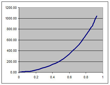
The only thing that has changed here is the X-axis scale.

Step 4. Find the polynomial

This could be hard, but Excel makes it easy.

• Click on the chart so the actual curve is selected.
• In the Chart menu select Add Trendline (this may vary with different versions of Excel. I still happily use Excel 97).
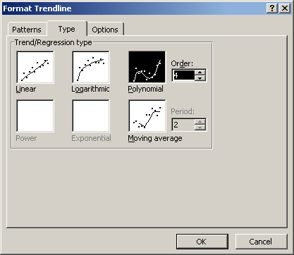
• In the trendline dialog box, select type = Polynomial and click the Order up to 4 (the latter may change later)
  
  
  
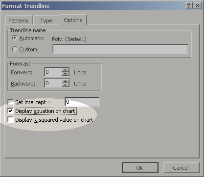
• In options select Display Equation on Chart
  
  
  
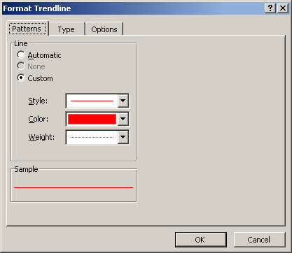
• In Patterns select the lightest line weight and a contrasting color.
  
  
  
• Hit OK. You should now have something like this:
  
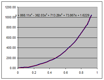
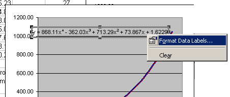
• Can you see the fancy equation? That’s what we are after. If you right-click the equation you can change the number formatting via Format Data labels
  
  
  
  A good choice is Scientific with about 7 digits precision: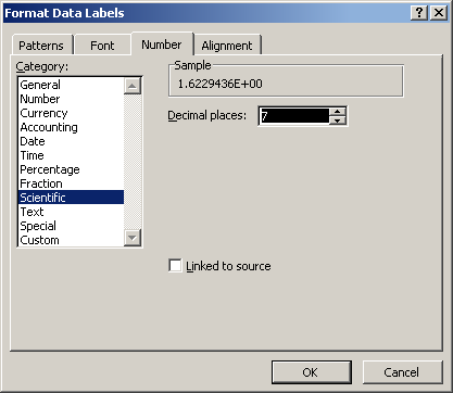
  
  
  Which should look like this: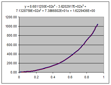
  
  
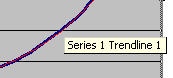
  (I moved the equation up and compressed the chart area down a bit by clicking on them and dragging the handles).
• Now move your mouse back over the the curve and shift it around until you get a tool tip that says Series 1 Trendline 1.
  
  
  
  Right click at that point. This will give you a context menu that will let you get back the Format Trendline dialog box with the Type tab. Try changing the Order of the polynomial. Lower orders, say 2, will not produce a trendline that fits the real data curve as well. Higher orders will give a better fit. My version of Excel maxes out at 6th order. The trade off is that a higher order polynomial will take SPLat longer to calculate.

Step 5. Identify the “polynomial coefficients”

The coefficients are the number that appear in front of (as multipliers for) the powers of x.

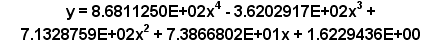
Here the “4th order coefficient” is 8.6811250E+02. With a little practice you can learn to highlight individual coefficients with your mouse, copy them and paste directly into your SPLat program. Just be aware that Excel adds a space after the minus signs. You must reproduce the minus signs correctly, without a space after them.

Step 6. Use the example code:

Program examples are no longer installed with SPLat/PC. They are now located on our website in the File Resources area. In folder examples\math\poly\ is a program polygen.spt. polygen.spt contains a general purpose polynomial calculator.

The calculator gets its coefficient from a table. All you have to do is build a table of coefficients and point the code to it. The comments in the program show you how to do this.

Other uses

This technique can be used to generate otherwise difficult mathematical functions like trig functions, logs and exponentials. The key to success is to limit the input numbers (arguments) to the narrowest possible range.

• Only cater for the range of numbers that will actually occur in your application, no more.
• Use known mathematical relationships like sin(90+x)=sin(90-x) and sin(-x)= -sin(x) (in degrees). With logs you can multiply an argument by a known constant, say 0.1 or 10, take the log and then add the log of the constant.